Solid stability and periodic elastic properties

These experimental public workflows add linear initial-stress buckling and small-strain periodic homogenization. They do not implement a special column solver or a special negative-Poisson-ratio material law.

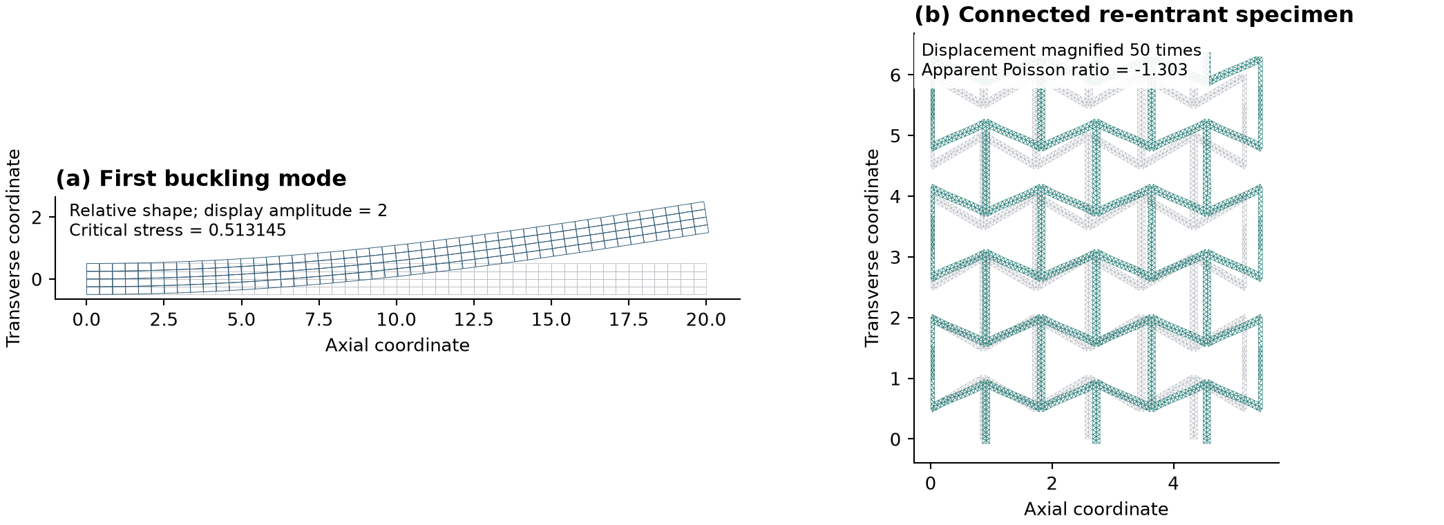
Linear buckling

Create studies.buckling_solid(dimension=2, assumption="plane_stress") (or plane strain / 3D), register displacement and elastic materials, and define homogeneous perturbation supports. Solve the reference loading separately with an ordinary static model on the same mesh and material partition. Then:

result = model.step(
    target=u,
    reference_displacement=u_reference,
    reference_name="uniform compressive traction: 1 stress unit",
    modes=3,
).solve_result(output="buckling.xdmf", strict_output=True)
load_factors = result.quantity("load_factors")

An optional base_displacement=..., base_name=... represents a fixed load that is not multiplied by the load factor. The pencil is

\[ (K+K_G(u_b)+\lambda K_G(u_r))\phi=0. \]

operators.geometric_stiffness(target, stress) owns the initial-stress form. Tension-positive stress means compression destabilizes. Both matrices use identical free-DOF elimination. The SLEPc backend uses GNHEP with shift-invert near zero: the geometric matrix may be indefinite or singular, and is not assumed to be a positive-definite modal mass matrix. Positive real factors are selected; an insufficient accepted spectrum raises an error. Modes have maximum absolute nodal component one and deterministic sign. Their amplitudes are relative, not a physical initial imperfection. Repeated modes can rotate within an eigenspace.

The reference and base fields are copied at Step construction. The caller is responsible for their equilibrium and matching material assumptions; naming a state alone does not prove equilibrium. The fixed base must remain stable and small-displacement. This is not a finite-deformed-base perturbation method. Only conservative elastic solids and strong supports are covered. Follower loads, MPC buckling, contact, plasticity and shells remain outside this delivery. Bounded mode-imperfection, displacement-control and serial spherical arc-length workflows are described below.

Periodic elastic properties

Use a load-free studies.static_solid model, registered elastic materials and one displacement field for the periodic fluctuation. Multi-material partitions must share tags: use mesh.partition_cells(...).

result = mechanics.periodic_elasticity(model, fluctuation, anchor=(0., 0.))
C = result.quantity("effective_stiffness")
E = result.quantity("young_moduli")
nu = result.quantity("poisson_ratios")

The geometry is a complete rectangular cell envelope with a matching-node mesh of its solid phase. The anchor is one solid node, not a maximum-face slave. Three 2D or six 3D engineering-strain basis cases are solved through ordinary model.step(...). The strain order is xx, yy, xy in 2D and xx, yy, zz, yz, xz, xy in 3D. Shear strain is engineering shear; shear stress is the tensor component. All stresses and energies are normalized by the complete cell envelope, including void space.

From compliance S=C^-1, E_i=1/S_ii and nu_ij=-S_ji/S_ii, where i is the loading direction and j is the transverse direction. No isotropy is assumed. Plane-strain properties describe the constrained in-plane response rather than the unconstrained 3D Young modulus. Negative directional Poisson ratios below -1 can be admissible for anisotropic structures.

Every case records periodic mismatch, reduced-equilibrium residual and Hill–Mandel energy mismatch; the matrix retains its measured symmetry error instead of being silently symmetrized. Failed consistency or singular/unstable stiffness blocks property publication.

Exact assembled-matrix projection

The workflow explicitly selects LinearSolverOptions(mpc_assembly="algebraic"). It consumes the existing rectangular MPC graph but forms T.T @ A @ T from the ordinary assembled operator. Numerical matrices remain distributed; root/constraint numbering is replicated, so extreme-scale graph construction is not claimed. One unit master per slave and homogeneous essential constraints are required. The existing mpc_assembly="native" default remains unchanged elsewhere.

On the local FEniCSx 0.11 stack, the re-entrant example exposed an approximately 0.9% difference between the native MPC route and explicit algebraic projection, despite satisfied periodic relations. The native route had a maximum Hill–Mandel error around 1.3%; explicit projection reduced it to about 2e-12. This is a reproducible local observation, not a claim that all upstream MPC versions or formulations are defective. The independent assembled projection is therefore used for this new homogenization workflow.

Geometry and finite specimens

mesh.reentrant_honeycomb(...) returns a normal mesh and tags, not a solver. Angle, inclined/vertical ligament length, thickness, repeats and mesh size are parameters. Default periodic clipping preserves boundary fragments that are connected through the periodic cell. connected_specimen=True retains the largest connected solid component and removes detached cut fragments for an ordinary finite specimen. This intentional geometric difference is explicit. The generator restores a caller's active Gmsh model and mesh-size options.

mechanics.apparent_poisson_ratio(...) measures finite-specimen strains using area-averaged displacements on four named gauge boundaries and explicit gauge lengths. It rejects near-zero axial strain. It does not label a finite array's apparent response as a periodic effective property. Applications can provide other geometries and gauge regions without modifying the solver.

Reproducible acceptance

• examples/linear_buckling_column/case.py: actual static reference solve, three modes, XDMF output, Euler reference. A length-20, unit-depth, E=1000, nu=0 cantilever gives critical stress about 0.513145 versus Euler 0.514042 (0.175% difference). Solid and beam theories need not converge to exactly the same value at finite slenderness.
• examples/reentrant_honeycomb/case.py: periodic cell and connected 3x3 finite specimen, named gauges and support reactions. For this geometry, periodic nu_xy is approximately -1.433, finite-array apparent nu_xy -1.303. These are computed predictions, not experimental validation.
• tests/test_stability_periodic.py: Euler cantilever and pin–roller supports, reference-load and length scaling, fixed-base superposition, 2D/3D agreement, solid-cell parameter recovery, two-material series/parallel reference, negative-Poisson cell, amplitude independence, energy and gauge checks.
• tests/stability_periodic_evidence_driver.py: mesh refinement records in evidence/stability_periodic/2026-10-10.json. Refining the honeycomb from h=0.07 to 0.04 changes nu_xy by about 0.011%, but shear stiffness still changes about 1.6%; do not infer all-observable mesh convergence from nu alone.

Run in fenicsx-env; MPI acceptance uses the same tests with two ranks. The honeycomb requires optional Gmsh and the periodic graph requires dolfinx_mpc.

Next isolated increments

1. Extend the bounded imperfection and displacement-control workflow to more geometry orders, materials and independent postbuckling references.
2. Distributed and transaction-aware adapters for the new sparse continuation core; retain the independently validated cohesive-specific path.
3. Oblique/nonmatching periodic cells and large-strain response as separate extensions, sharing the existing field, state and output contracts.

References

• FEniCSx solid buckling derivation
• SLEPc eigenproblem types
• FEniCSx periodic elasticity
• Abaqus eigenvalue buckling
• COMSOL homogenization

Mode imperfections and displacement-controlled response

An additional bounded workflow is now provided by examples/imperfect_column. The existing displacement-based neo-Hookean solver already provides consistent tangents, adaptive increments, failed-attempt rollback and accepted snapshots; this workflow reuses it rather than introducing another nonlinear solver.

receipt = mesh.apply_mode_imperfection(
    domain, [buckling_result.field("Buckling_mode_1")], amplitudes=[0.02]
)
# Build a fresh nonlinear model on the perturbed, stress-free geometry.
# Keep moving boundaries through tagged_boundary_region, not old x==L predicates.
# After the ordinary model.step(...).solve_result():
curve = mechanics.displacement_controlled_response(model, step, on=loaded_end)
# receipt.restore() restores original coordinates when the deformed model is no longer used.

Amplitudes have length units. Each mode is normalized by its maximum vector norm at geometry nodes; multiple signed amplitudes can be combined. Original geometry is retained in the receipt. Failed quality/orientation checks restore coordinates. The current scope is full-dimensional linear-coordinate triangle, quadrilateral, tetrahedron and hexahedron meshes; displacement/mode fields may be higher order. Do not reuse assembled operators or geometric search trees after a geometry edit.

Curve extraction currently supports ordinary strong-boundary, single-material hyperelastic displacement loading, without body/traction loads, eigenstrains or boundary models. Reaction and monitor displacement are signed; the example plots compression and shortening as positive. Measurements use the reference boundary area, not a nodal-average surrogate. Save every accepted increment for a complete accepted-step curve. This is not a general arc-length or snap-back algorithm.

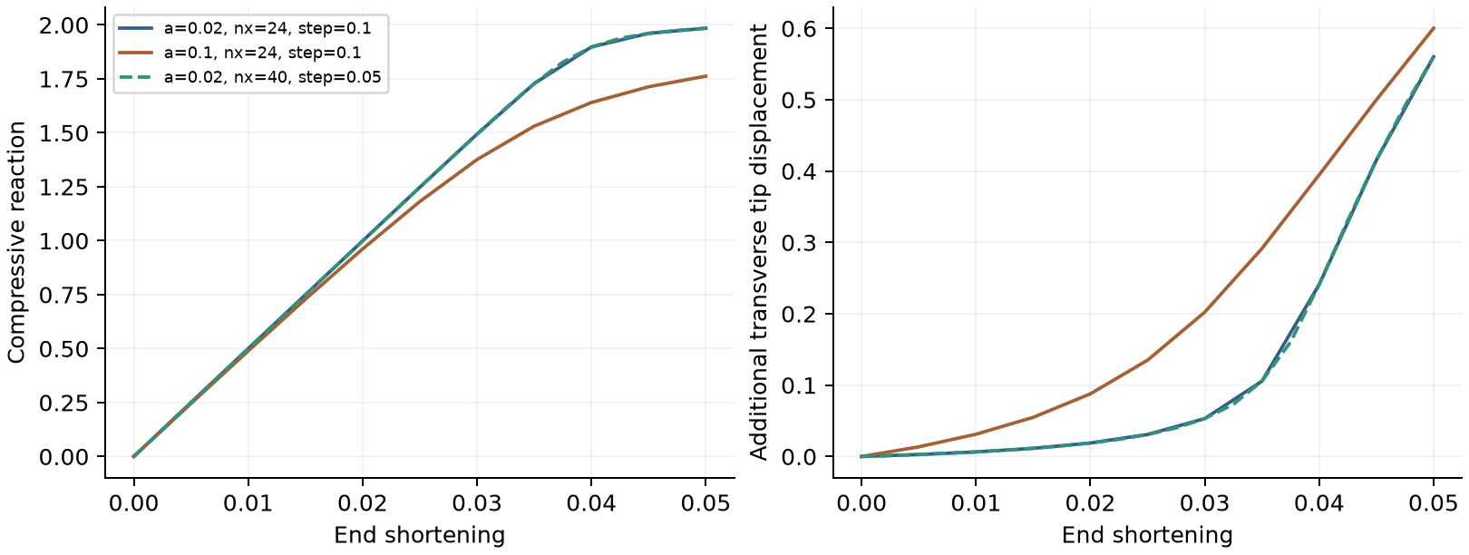
For the guided-end example, at shortening 0.05, increasing initial amplitude from 0.02 to 0.10 changes compression force from 1.98445 to 1.76232. Refining nx=24 to 40 and halving maximum increment changes the small-imperfection final force by about 0.010% and transverse displacement by about 0.017%. These are internal refinement checks, not independent commercial-software validation.

Sparse spherical arc-length continuation

The physics-independent solvers.ArcLengthPath consumes an internal-force and consistent-tangent callback, a reference load vector, and optionally a fixed load:

\[ \mathbf r(\mathbf u,\lambda) =\mathbf f_{\rm int}(\mathbf u)-\mathbf f_0-\lambda\mathbf f_{\rm ref}=0. \]

Here u denotes the free unknowns, lambda the load multiplier, f0 the fixed load, and fref the scalable reference load. The accepted displacement/load increment is constrained by

\[ g=\frac{1}{n}\sum_{i=1}^n\left(\frac{\Delta u_i}{u_*}\right)^2 +\left(\frac{\Delta\lambda}{\lambda_*}\right)^2-\Delta s^2=0. \]

The user declares positive displacement and load scales u* and lambda*; n is the number of free unknowns and delta-s the dimensionless arc length. RMS scaling reduces the trivial dependence on the number of unknowns, but is not a spatial mass-matrix metric or a guarantee of mesh-independent stepping. Changing scales changes sampling of a path, not its equilibrium equation.

The corrector solves the bordered Newton system for displacement and load simultaneously, using K = derivative of fint with respect to u:

\[ \begin{bmatrix} \mathbf K &-\mathbf f_{\rm ref}\\ 2\Delta\mathbf u^T\mathbf W &2\Delta\lambda/\lambda_*^2 \end{bmatrix} \begin{bmatrix}\delta\mathbf u\\\delta\lambda\end{bmatrix} =-\begin{bmatrix}\mathbf r\\g\end{bmatrix}, \qquad W_{ii}=1/(n u_*^2). \]

It does not require inversion of K at a limit point. A tangent predictor is oriented using the previous accepted increment; failed correctors reduce the arc length while retaining the accepted state. Both force equilibrium and the arc constraint must converge. Callbacks must be stateless: irreversible material commit/rollback belongs to a future transaction-aware adapter. This algorithm is a spherical method, not a claim of reproducing Abaqus modified Riks exactly.

The first FEniCSx adapter is available through the ordinary public Step route:

step = model.step(
    target=u,
    procedure=procedures.arc_length(),
    arc_options=solvers.ArcLengthOptions(
        initial=0.04, maximum=0.04,
        displacement_scale=0.2, load_scale=0.1,
    ),
    increments=80,
)
result = step.solve_result()
frame = step.displacement_at(20)  # copy of zero-based accepted increment

This adapter supports serial 2D/3D displacement-based hyperelasticity, homogeneous strong supports, and proportional dead body forces/tractions. No follower pressures, independent load amplitudes, contact, MPC, nonzero prescribed-displacement paths, plasticity or irreversible damage are included. Distributed execution is rejected explicitly rather than silently gathering a large model. Reference coefficients must remain fixed during the analysis. An initially equilibrated generic algebraic state can include a fixed load; the first FE adapter starts at zero reference load without a separate preload.

Verification includes an analytical two-bar shallow arch (including load reversal), 2D/3D homogeneous hyperelastic patches, and the continuum solid arch below with mesh/step refinement. The solid arch crosses two load limit points; no automatic bifurcation branch switching is claimed. Its static descending branch must not be mistaken for a time-resolved snap-through trajectory.

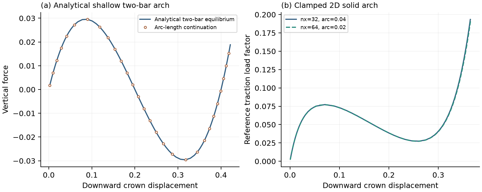
See examples/shallow_arch_arc_length, tests/test_arc_length.py and evidence/stability_periodic/arc_length.json for reproducible results. The existing stateful cohesive-specific continuation remains unchanged. For the engineering distinction between static path following, proportional loading and dynamic collapse, see the Abaqus postbuckling guide.