From simulations to a surrogate model
A single finite-element result answers one question. A parameterized set of results can answer a family of questions—and become training data for a fast approximation. The difficult handoff is often not choosing a neural network; it is keeping track of what was varied, what was computed, and which results are suitable for learning.
AgentFEM's small elasticity campaign makes that handoff explicit.
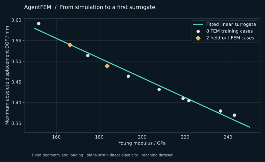
Ten FEM cases, eight for fitting and two held out. This teaching run used AgentFEM 0.3.3 and DOLFINx 0.11.0. The line is a scalar linear baseline, not a neural operator.
The physical problem
A two-dimensional, plane-strain cantilever is fixed on the left and loaded by a downward traction on the right. Geometry, mesh, Poisson ratio, and traction remain unchanged. The Young modulus varies from 150 to 250 GPa.
The output is the global maximum absolute displacement degree of freedom, in metres. It is not silently substituted with the maximum displacement-vector magnitude or a selected tip displacement.
Run the existing example
Want to try the learning step first, without installing a FEM runtime? The standalone NumPy mini-lab includes the ten FEM outputs, fitting code, units, and provenance. The community discussion suggests a small physics-based feature experiment.
The notebook compares two simple feature choices and lets you change the material stiffness. It uses the published FEM data, NumPy, and Matplotlib; no finite-element installation is needed for this learning step. Colab may request sign-in to start its runtime. You can also download the notebook from the mini-lab and run it locally in Jupyter.
Use an installed, compatible AgentFEM environment and a matching source checkout; the repository example is not bundled as an executable script in every package installation. From that checkout's root:
The default run uses ten Latin-hypercube samples with a fixed seed. It builds a fresh model for each sample, solves with FEniCSx, applies the declared result policy, and assembles a scientific dataset. A ridge baseline then uses a training/validation split and reports its validation result.
Young modulus → finite-element cases → accepted dataset
              → ridge fit → held-out validation → guarded prediction
What the example produces
Under examples_output/static_elasticity_surrogate_campaign/:
| Directory | What it preserves |
|---|---|
campaign/ |
Case execution records and campaign artifacts |
trusted_dataset/ |
Inputs, declared output values, units, and dataset metadata |
surrogate/ |
The fitted model artifact and associated model information |
The terminal reports validation metrics and the source of the final prediction. The example's configured relative-L2 threshold is 5%; that is an acceptance condition for this demonstration, not a universal accuracy promise. With only ten cases, the holdout set is small: use this to learn the workflow, not to establish a broad engineering qualification.
Why begin without a neural network?
There is only one varying physical input here. A transparent baseline makes it easier to inspect the dataset and recognize errors before moving to a higher-dimensional problem. More elaborate models earn their place when the geometry, spatial fields, loading history, or other inputs warrant them.
AgentFEM provides optional PyTorch integration and user-owned estimator interfaces. The learning companion adds maintained scientific-learning providers. A neural operator that maps fields to fields is a different modeling choice from this scalar surrogate.
Scale the workflow, not the claims
For a new application, first define the inputs, units, output quantity, and usable parameter range. Then add appropriate sampling, independent test cases, and a failure policy. The example's guard can fall back to a new FEM solve when a requested parameter is outside the surrogate's domain.
Campaign and dataset reference · Simulation-to-learning guide · Explore more cases